Multivariate normal distribution

This examples shows the use of the multivariate normal distributions class. In particular:

• How to define one of the univariate distributions supported by UQpy

• How to plot the pdf of the distribution

• How to extract the moments of the distribution

• How to draw random samples from the distribution

Initially we have to import the necessary modules.

import numpy as np
import matplotlib.pyplot as plt
from UQpy.distributions.collection.MultivariateNormal import MultivariateNormal

Example of a multivariate normal distribution

Note that multivariate normal distribution can facilitate any number of dimensions. In order to define it two arguments are necessary, specifically, a list containing the mean values for each one of the dimensions and a covariance matrix with shape (ndimensions, ndimensions)

print(MultivariateNormal.__bases__)
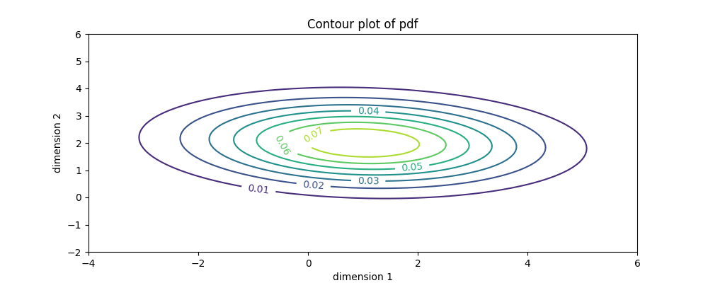
dist = MultivariateNormal(mean=[1., 2.], cov=[[4., -0.2], [-0.2, 1.]])

(<class 'UQpy.distributions.baseclass.DistributionND.DistributionND'>,)

Plot the two-dimensional pdf of the distribution.

fig, ax = plt.subplots(ncols=1, figsize=(10, 4))
x = np.arange(-6.0, 6.0, 0.1)
y = np.arange(-6.0, 6.0, 0.1)
X, Y = np.meshgrid(x, y)
Z = dist.pdf(x=np.concatenate([X.reshape((-1, 1)), Y.reshape((-1, 1))], axis=1))
CS = ax.contour(X, Y, Z.reshape(X.shape))
ax.clabel(CS, inline=1, fontsize=10)
ax.set_xlabel('dimension 1')
ax.set_ylabel('dimension 2')
ax.set_title('Contour plot of pdf')
ax.set_xlim([-4, 6])
ax.set_ylim([-2, 6])
plt.show()

Print the multivariate moments of the distribution.

Providing a single or multiple consecutive initials of the following four distributions moments

• ‘m’: mean

• ‘v’: variance

• ‘s’: skewness

• ‘k’: kurtosis

allows the user to obtain the respective moments from all underlying univariate distributions. In the following examples providing the string ‘mv’ to the moments function, returns the respective means and variances.

print(dist.moments())
print(dist.moments(moments2return='mv'))

([1.0, 2.0], [[4.0, -0.2], [-0.2, 1.0]])
([1.0, 2.0], [[4.0, -0.2], [-0.2, 1.0]])

Generate 1000 random samples from the binomial distribution.

Important: the output of rvs is a (nsamples, 1) ndarray.

data = dist.rvs(nsamples=1000)

fig, ax = plt.subplots(ncols=1, figsize=(10, 4))
ax.scatter(data[:, 0], data[:, 1], alpha=0.2)
ax.set_xlabel('dimension 1')
ax.set_ylabel('dimension 2')
ax.set_title('random samples')
ax.set_xlim([-4, 6])
ax.set_ylim([-2, 6])

(-2.0, 6.0)