Rosenbrock performance function

1. Import the necessary libraries

import matplotlib.pyplot as plt
import numpy as np
import scipy.stats as stats

from UQpy import PythonModel
# Import this newly defined Rosenbrock distribution into the Distributions module
from UQpy.distributions import Normal
from UQpy.reliability import SubsetSimulation
from UQpy.run_model.RunModel import RunModel
from UQpy.sampling import ModifiedMetropolisHastings, Stretch
# First import the file that contains the newly defined Rosenbrock distribution
from local_Rosenbrock import Rosenbrock

ModifiedMetropolisHastings Initial Samples

m = PythonModel(model_script='local_Rosenbrock_pfn.py', model_object_name="RunPythonModel")
model = RunModel(model=m)
dist = Rosenbrock(p=100.)
dist_prop1 = Normal(loc=0, scale=1)
dist_prop2 = Normal(loc=0, scale=10)

x = stats.norm.rvs(loc=0, scale=1, size=(100, 2), random_state=83276)

mcmc_init1 = ModifiedMetropolisHastings(dimension=2, log_pdf_target=dist.log_pdf, seed=x.tolist(),
                                                           burn_length=1000, proposal=[dist_prop1, dist_prop2],
                                                           random_state=8765)
mcmc_init1.run(10000)

sampling=Stretch(log_pdf_target=dist.log_pdf, dimension=2, n_chains=1000, random_state=38546)
x_ss_MMH = SubsetSimulation(sampling=sampling, runmodel_object=model, conditional_probability=0.1,
                            nsamples_per_subset=10000, samples_init=mcmc_init1.samples)

for i in range(len(x_ss_MMH.performance_function_per_level)):
    plt.scatter(x_ss_MMH.samples[i][:, 0], x_ss_MMH.samples[i][:, 1], marker='o')
plt.grid(True)
plt.xlabel(r'$X_1$')
plt.ylabel(r'$X_2$')
plt.yticks(np.arange(-20, 180, step=20))
plt.xlim((-10, 15))
plt.tight_layout()
plt.show()


print(x_ss_MMH.failure_probability)

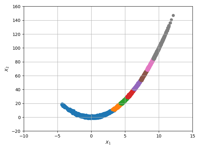
4.0450000000000015e-08

Stretch Initial Samples

m = PythonModel(model_script='local_Rosenbrock_pfn.py', model_object_name="RunPythonModel")
model = RunModel(model=m)
dist = Rosenbrock(p=100.)

x = stats.norm.rvs(loc=0, scale=1, size=(100, 2), random_state=83276)

mcmc_init2 = Stretch(dimension=2, log_pdf_target=dist.log_pdf, seed=x.tolist(),
                                                burn_length=1000, random_state=8765)
mcmc_init2.run(10000)

sampling=Stretch(log_pdf_target=dist.log_pdf, dimension=2, n_chains=1000, random_state=83456)
x_ss_Stretch = SubsetSimulation(sampling=sampling, runmodel_object=model, conditional_probability=0.1,
                                nsamples_per_subset=10000, samples_init=mcmc_init2.samples)

for i in range(len(x_ss_Stretch.performance_function_per_level)):
    plt.scatter(x_ss_Stretch.samples[i][:, 0], x_ss_Stretch.samples[i][:, 1], marker='o')
plt.grid(True)
plt.xlabel(r'$X_1$')
plt.ylabel(r'$X_2$')
plt.yticks(np.arange(-20, 180, step=20))
plt.xlim((-10, 15))
plt.tight_layout()
plt.show()

print(x_ss_Stretch.failure_probability)


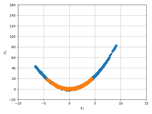
plt.figure()
plt.plot(mcmc_init2.samples[:, 0], mcmc_init2.samples[:, 1], 'o')
plt.plot(mcmc_init1.samples[:, 0], mcmc_init1.samples[:, 1], 'x')
plt.grid(True)
plt.xlabel(r'$X_1$')
plt.ylabel(r'$X_2$')
plt.yticks(np.arange(-20, 180, step=20))
plt.xlim((-10, 15))
plt.tight_layout()
plt.show()

• 
• 

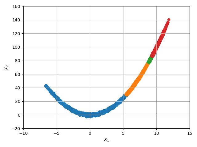
0.0004715000000000001