Gaussian Process with noisy output

This jupyter script shows the performance of GaussianProcessRegressor class in the UQpy. A training data is generated using a function (\(f(x)\), as defined below), which is used to train a surrogate model.

Import the necessary modules to run the example script. Notice that FminCobyla is used here, to solve the MLE optimization problem with constraints.

import numpy as np
import matplotlib.pyplot as plt
import warnings

from UQpy.utilities import RBF

warnings.filterwarnings('ignore')
from UQpy.utilities.MinimizeOptimizer import MinimizeOptimizer
from UQpy.surrogates.gaussian_process.regression_models.LinearRegression import LinearRegression
from UQpy.surrogates import GaussianProcessRegression

Consider the following function \(f(x)\).

\[f(x) = \frac{1}{100} + \frac{5}{8}(2x-1)^4[(2x-1)^2 + 4\sin{(5 \pi x)^2}], \quad \quad x \in [0,1]\]

def funct(x):
    y = (1 / 100) + (5 / 8) * ((2 * x - 1) ** 4) * (((2 * x - 1) ** 2) + 4 * np.sin(5 * np.pi * x) ** 2)
    return y

Define the training data set. The following 13 points have been used to fit the GP.

X_train = np.array([0, 0.06, 0.08, 0.26, 0.27, 0.4, 0.52, 0.6, 0.68, 0.81, 0.9, 0.925, 1]).reshape(-1, 1)
y_train = funct(X_train)

Define the test data.

X_test = np.linspace(0, 1, 100).reshape(-1, 1)
y_test = funct(X_test)

Train GPR

• Noise

• No Constraints

Define kernel used to define the covariance matrix. Here, the application of Radial Basis Function (RBF) kernel is demonstrated.

kernel2 = RBF()

Define the optimizer used to identify the maximum likelihood estimate.

bounds_2 = [[10**(-3), 10**3], [10**(-3), 10**2], [10**(-3), 10**(2)]]
optimizer2 = MinimizeOptimizer(bounds=bounds_2)

Define the ‘GaussianProcessRegressor’ class object, the input attributes defined here are kernel, optimizer, initial estimates of hyperparameters and number of times MLE is identified using random starting point.

gpr2 = GaussianProcessRegression(kernel=kernel2, hyperparameters=[1, 1, 0.1], optimizer=optimizer2,
                                 optimizations_number=10, noise=True, regression_model=LinearRegression())

Call the ‘fit’ method to train the surrogate model (GPR).

gpr2.fit(X_train, y_train)

The maximum likelihood estimates of the hyperparameters are as follows:

print(gpr2.hyperparameters)

print('Length Scale: ', gpr2.hyperparameters[0])
print('Process Variance: ', gpr2.hyperparameters[1])
print('Noise Variance: ', gpr2.hyperparameters[2])

[0.07355891 0.50023891 0.001     ]
Length Scale:  0.07355891429773363
Process Variance:  0.5002389052315005
Noise Variance:  0.001

Use ‘predict’ method to compute surrogate prediction at the test samples. The attribute ‘return_std’ is a boolean indicator. If ‘True’, ‘predict’ method also returns the standard error at the test samples.

y_pred2, y_std2 = gpr2.predict(X_test, return_std=True)

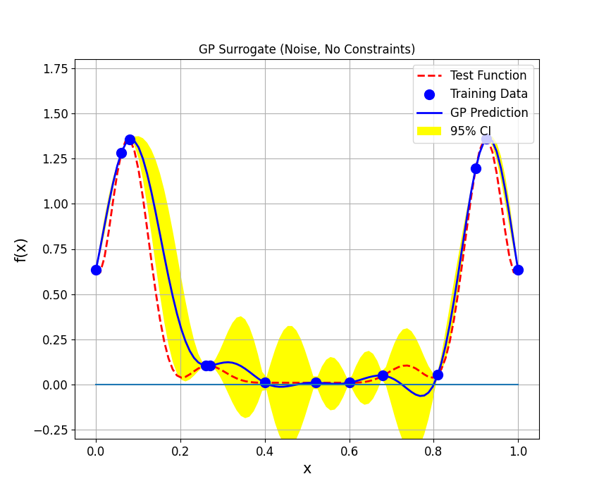
The plot shows the test function in dashed red line and 13 training points are represented by blue dots. Also, blue curve shows the GPR prediction for $x in (0, 1)$ and yellow shaded region represents 95% confidence interval.

fig, ax = plt.subplots(figsize=(8.5,7))
ax.plot(X_test,y_test,'r--',linewidth=2,label='Test Function')
ax.plot(X_train,y_train,'bo',markerfacecolor='b', markersize=10, label='Training Data')
ax.plot(X_test,y_pred2,'b-', lw=2, label='GP Prediction')
ax.plot(X_test, np.zeros((X_test.shape[0],1)))
ax.fill_between(X_test.flatten(), y_pred2-1.96*y_std2,
                y_pred2+1.96*y_std2,
                facecolor='yellow',label='95% CI')
ax.tick_params(axis='both', which='major', labelsize=12)
ax.set_xlabel('x', fontsize=15)
ax.set_ylabel('f(x)', fontsize=15)
ax.set_ylim([-0.3,1.8])
plt.title('GP Surrogate (Noise, No Constraints)')
ax.legend(loc="upper right",prop={'size': 12});
plt.grid()
plt.show()