Gaussian Process of a sinusoidal function

In this example, Gaussian Process Regression is used to generate a surrogate model for a given data. In this data, sample points are generated using TrueStratifiedSampling class and functional value at sample points are estimated using a model defined in python script (‘python_model_function.py).

Import the necessary libraries. Here we import standard libraries such as numpy and matplotlib, but also need to import the TrueStratifiedSampling, RunModel and GaussianProcessRegression class from UQpy.

import shutil

from UQpy import PythonModel
from UQpy.sampling.stratified_sampling.strata import RectangularStrata
from UQpy.sampling import TrueStratifiedSampling
from UQpy.run_model.RunModel import RunModel
from UQpy.distributions import Gamma
import numpy as np
import matplotlib.pyplot as plt
from UQpy.surrogates import GaussianProcessRegression

Create a distribution object.

from UQpy.utilities import RBF

marginals = [Gamma(a=2., loc=1., scale=3.)]

Create a distribution object.

strata = RectangularStrata(strata_number=[20])

Run stratified sampling

x = TrueStratifiedSampling(distributions=marginals, strata_object=strata,
                           nsamples_per_stratum=1, random_state=2)

RunModel is used to evaluate function values at sample points. Model is defined as a function in python file ‘python_model_function.py’.

model = PythonModel(model_script='local_python_model_1Dfunction.py', model_object_name='y_func',
                    delete_files=True)
rmodel = RunModel(model=model)
rmodel.run(samples=x.samples)

from UQpy.surrogates.gaussian_process.regression_models import LinearRegression
from UQpy.utilities.MinimizeOptimizer import MinimizeOptimizer

bounds = [[10**(-3), 10**3], [10**(-3), 10**2]]
optimizer = MinimizeOptimizer(method='L-BFGS-B', bounds=bounds)

K = GaussianProcessRegression(regression_model=LinearRegression(), kernel=RBF(),
                              optimizer=optimizer, optimizations_number=20, hyperparameters=[1, 0.1],
                              random_state=2)
K.fit(samples=x.samples, values=rmodel.qoi_list)
print(K.hyperparameters)

[2.62770035 1.5096804 ]

RunModel is used to evaluate function values at sample points. Model is defined as a function in python file ‘python_model_function.py’.

num = 1000
x1 = np.linspace(min(x.samples), max(x.samples), num)

y, y_sd = K.predict(x1.reshape([num, 1]), return_std=True)

Actual model is evaluated at all points to compare it with kriging surrogate.

rmodel.run(samples=x1, append_samples=False)

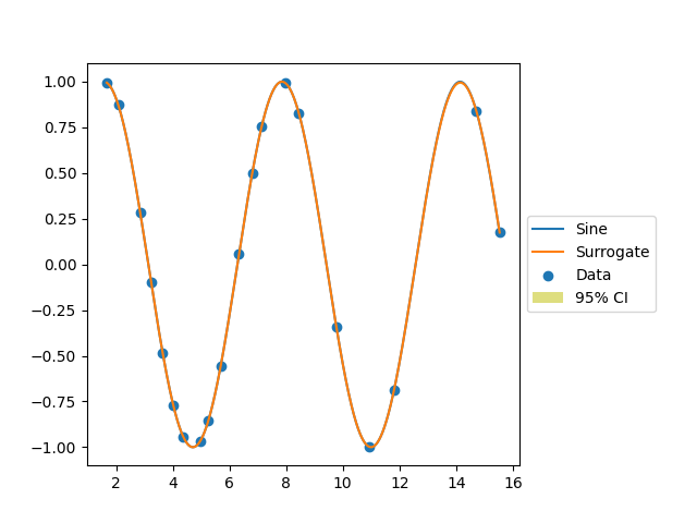
This plot shows the input data as blue dot, blue curve is actual function and orange curve represents response curve. This plot also shows the gradient and 95% confidence interval of the kriging surrogate.

fig = plt.figure()
ax = plt.subplot(111)
plt.plot(np.squeeze(x1), np.squeeze(rmodel.qoi_list), label='Sine')
plt.plot(x1, y, label='Surrogate')
# plt.plot(x1, y_grad, label='Gradient')
plt.scatter(K.samples, K.values, label='Data')
plt.fill(np.concatenate([x1, x1[::-1]]), np.concatenate([y - 1.9600 * y_sd,
                                                         (y + 1.9600 * y_sd)[::-1]]),
         alpha=.5, fc='y', ec='None', label='95% CI')
box = ax.get_position()
ax.set_position([box.x0, box.y0, box.width * 0.8, box.height])

# Put a legend to the right of the current axis
ax.legend(loc='center left', bbox_to_anchor=(1, 0.5))
plt.show()