Kernel

This example shows how to use the UQpy Grassmann class to compute kernels

Import the necessary libraries. Here we import standard libraries such as numpy and matplotlib, but also need to import the Grassmann class from UQpy implemented in the DimensionReduction module.

import numpy as np
import matplotlib
import matplotlib.pyplot as plt
from mpl_toolkits.axes_grid1 import make_axes_locatable
from UQpy.dimension_reduction.grassmann_manifold.projections.SVDProjection import SVDProjection
from UQpy.dimension_reduction import GrassmannOperations
from UQpy.utilities import GrassmannPoint
from UQpy.utilities.kernels import ProjectionKernel
import sys

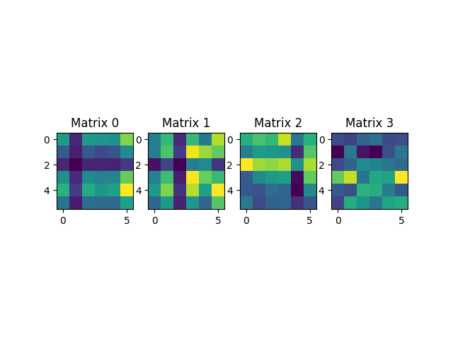
Generate four random matrices with reduced rank corresponding to the different samples. The samples are stored in matrices.

D1 = 6
r0 = 2  # rank sample 0
r1 = 3  # rank sample 1
r2 = 4  # rank sample 2
r3 = 3  # rank sample 2

np.random.seed(1111)  # For reproducibility.
# Solutions: original space.
Sol0 = np.dot(np.random.rand(D1, r0), np.random.rand(r0, D1))
Sol1 = np.dot(np.random.rand(D1, r1), np.random.rand(r1, D1))
Sol2 = np.dot(np.random.rand(D1, r2), np.random.rand(r2, D1))
Sol3 = np.dot(np.random.rand(D1, r3), np.random.rand(r3, D1))

# Creating a list of solutions.
matrices = [Sol0, Sol1, Sol2, Sol3]

# Plot the solutions
fig, (ax1, ax2, ax3, ax4) = plt.subplots(1, 4)
ax1.title.set_text('Matrix 0')
ax1.imshow(Sol0)
ax2.title.set_text('Matrix 1')
ax2.imshow(Sol1)
ax3.title.set_text('Matrix 2')
ax3.imshow(Sol2)
ax4.title.set_text('Matrix 3')
ax4.imshow(Sol3)
plt.show()

Instantiate the SvdProjection class that projects the raw data to the manifold.

manifold_projection = SVDProjection(matrices, p="max")

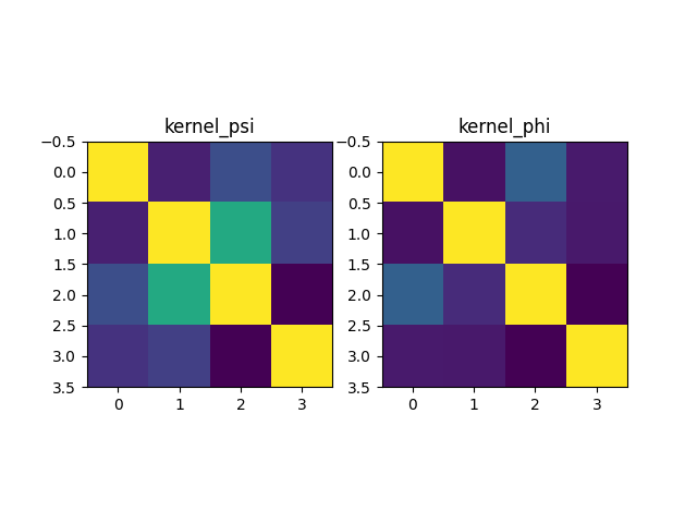
Compute the kernels for \(\Psi\) and \(\Phi\), the left and right -singular eigenvectors, respectively, of singular value decomposition of each solution.

projection_kernel = ProjectionKernel()

projection_kernel.calculate_kernel_matrix(x=manifold_projection.u, s=manifold_projection.u)
kernel_psi = projection_kernel.kernel_matrix

projection_kernel.calculate_kernel_matrix(x=manifold_projection.v, s=manifold_projection.v)
kernel_phi = projection_kernel.kernel_matrix

fig, (ax1, ax2) = plt.subplots(1, 2)
ax1.title.set_text('kernel_psi')
ax1.imshow(kernel_psi)
ax2.title.set_text('kernel_phi')
ax2.imshow(kernel_phi)
plt.show()

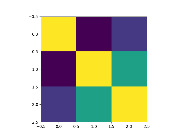
Compute the kernel only for 2 points.

projection_kernel.\
    calculate_kernel_matrix(x=[manifold_projection.u[0], manifold_projection.u[1], manifold_projection.u[2]],
                            s=[manifold_projection.u[0], manifold_projection.u[1], manifold_projection.u[2]])
kernel_01 = projection_kernel.kernel_matrix

fig = plt.figure()
plt.imshow(kernel_01)
plt.show()

Compute the kernels for \(\Psi\) and \(\Phi\), the left and right -singular eigenvectors, respectively, of singular value decomposition of each solution. In this case, use a user defined class UserKernel.

from UQpy.utilities.kernels.baseclass.GrassmannianKernel import GrassmannianKernel

class UserKernel(GrassmannianKernel):

    def element_wise_operation(self, xi_j) -> float:
        xi, xj = xi_j
        r = np.dot(xi.T, xj)
        det = np.linalg.det(r)
        return det * det


user_kernel = UserKernel()
user_kernel.calculate_kernel_matrix(x=manifold_projection.u, s=manifold_projection.u)
kernel_user_psi = user_kernel.kernel_matrix

user_kernel.calculate_kernel_matrix(x=manifold_projection.v, s=manifold_projection.v)
kernel_user_phi = user_kernel.kernel_matrix

fig, (ax1, ax2) = plt.subplots(1, 2)
ax1.title.set_text('kernel_psi')
ax1.imshow(kernel_user_psi)
ax2.title.set_text('kernel_phi')
ax2.imshow(kernel_user_phi)
plt.show()