2D Helmholtz eigenvalues (2 random inputs, vector-valued output)

In this example, PCE is used to generate a surrogate model for a given set of 2D data for a numerical model with multi-dimensional outputs.

Import necessary libraries.

import numpy as np
import matplotlib.pyplot as plt
import math
from UQpy.distributions import Normal, JointIndependent
from UQpy.surrogates import *

The analytical function below describes the eigenvalues of the 2D Helmholtz equation on a square.

def analytical_eigenvalues_2d(Ne, lx, ly):
    """
    Computes the first Ne eigenvalues of a rectangular waveguide with
    dimensions lx, ly

    Parameters
    ----------
    Ne : integer
         number of eigenvalues.
    lx : float
         length in x direction.
    ly : float
         length in y direction.

    Returns
    -------
    ev : numpy 1d array
         the Ne eigenvalues
    """
    ev = [(m * np.pi / lx) ** 2 + (n * np.pi / ly) ** 2 for m in range(1, Ne + 1)
          for n in range(1, Ne + 1)]
    ev = np.array(ev)

    return ev[:Ne]

Create a distribution object.

pdf_lx = Normal(loc=2, scale=0.02)
pdf_ly = Normal(loc=1, scale=0.01)
margs = [pdf_lx, pdf_ly]
joint = JointIndependent(marginals=margs)

Define the number of input dimensions and choose the number of output dimensions (number of eigenvalues).

dim_in = 2
dim_out = 10

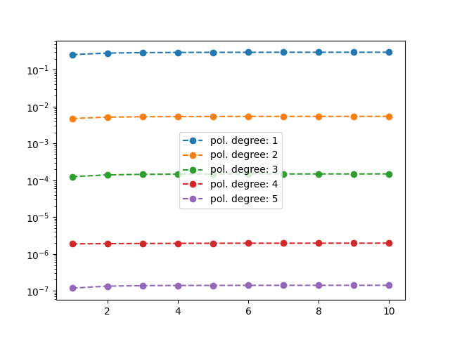
Construct PCE models by varying the maximum degree of polynomials (and therefore the number of polynomial basis) and compute the validation error for all resulting models.

errors = []
# construct PCE surrogate models
for max_degree in range(1, 6):
    print('Total degree: ', max_degree)
    polynomial_basis = TotalDegreeBasis(joint, max_degree)

    print('Size of basis:', polynomial_basis.polynomials_number)
    # training data
    sampling_coeff = 5
    print('Sampling coefficient: ', sampling_coeff)
    np.random.seed(42)
    n_samples = math.ceil(sampling_coeff * polynomial_basis.polynomials_number)
    print('Training data: ', n_samples)
    xx = joint.rvs(n_samples)
    yy = np.array([analytical_eigenvalues_2d(dim_out, x[0], x[1]) for x in xx])

    # fit model
    least_squares = LeastSquareRegression()
    pce_metamodel = PolynomialChaosExpansion(polynomial_basis=polynomial_basis, regression_method=least_squares)
    pce_metamodel.fit(xx, yy)

    # coefficients
    # print('PCE coefficients: ', pce.C)

    # validation errors
    np.random.seed(999)
    n_samples = 1000
    x_val = joint.rvs(n_samples)
    y_val = np.array([analytical_eigenvalues_2d(dim_out, x[0], x[1]) for x in x_val])
    y_val_pce = pce_metamodel.predict(x_val)
    errors.append(np.linalg.norm((y_val - y_val_pce) / y_val, ord=1, axis=0))
    print('Relative absolute errors: ', errors[-1])
    print('')

Total degree:  1
Size of basis: 3
Sampling coefficient:  5
Training data:  15
Relative absolute errors:  [0.25787331 0.28364754 0.29201537 0.29532324 0.29691008 0.29778109
 0.29831043 0.2986553  0.29889252 0.29906269]

Total degree:  2
Size of basis: 6
Sampling coefficient:  5
Training data:  30
Relative absolute errors:  [0.00475743 0.0051856  0.00531297 0.00536752 0.00539496 0.00541011
 0.00541937 0.00542546 0.00542968 0.00543271]

Total degree:  3
Size of basis: 10
Sampling coefficient:  5
Training data:  50
Relative absolute errors:  [0.00012562 0.00014033 0.00014521 0.00014706 0.00014794 0.00014842
 0.00014872 0.00014891 0.00014904 0.00014913]

Total degree:  4
Size of basis: 15
Sampling coefficient:  5
Training data:  75
Relative absolute errors:  [1.88728332e-06 1.90860554e-06 1.92961227e-06 1.94463745e-06
 1.95400955e-06 1.95956409e-06 1.96292959e-06 1.96512055e-06
 1.96687116e-06 1.96840806e-06]

Total degree:  5
Size of basis: 21
Sampling coefficient:  5
Training data:  105
Relative absolute errors:  [1.18499835e-07 1.34430527e-07 1.38327329e-07 1.39753722e-07
 1.40432776e-07 1.40809754e-07 1.41038037e-07 1.41186713e-07
 1.41288658e-07 1.41361880e-07]

Plot errors.

errors = np.array(errors)
plt.figure(1)
for i in range(np.shape(errors)[0]):
    plt.semilogy(np.linspace(1, dim_out, dim_out), errors[i], '--o', label='pol. degree: {}'.format(i+1))
plt.legend()
plt.show()

Moment estimation (directly estimated from the last PCE metamodel).

print('Mean PCE estimate:', pce_metamodel.get_moments()[0])
print('')
print('Variance PCE estimate:', pce_metamodel.get_moments()[1])

Mean PCE estimate: [ 12.34070845  41.95840874  91.32124256 160.4292099  249.28231077
 357.88054516 486.22391308 634.31241452 802.14604949 989.72481799]

Variance PCE estimate: [4.14672709e-02 6.26887565e-01 3.16370884e+00 9.99361227e+00
 2.43949515e+01 5.05827526e+01 9.37087143e+01 1.59861207e+02
 2.56065276e+02 3.90282635e+02]