Multivariate from independent marginals

This examples shows the use of the multivariate normal distribution class. In particular:

• How to define one multivariate distribution from independent marginals supported by UQpy

• How to plot the pdf of the distribution

• How to extract the moments of the distribution

• How to draw random samples from the distribution

Import the necessary modules.

from UQpy.distributions.collection import Normal, Lognormal, JointIndependent
import numpy as np
import matplotlib.pyplot as plt

Define a multivariate distribution from independent univariate marginals.

In order to define a JointIndependent distribution, a list of marginal distributions is initially created. These marginals are then provided as input to the JointIndependent class of UQpy. Retrieving the multivariate distribution parameters is achieved using the get_parameters method.

marginals = [Normal(loc=2., scale=2.),
             Lognormal(s=1., loc=0., scale=np.exp(5))]

dist = JointIndependent(marginals=marginals)

print(dist.get_parameters())

{'loc_0': 2.0, 'scale_0': 2.0, 's_1': 1.0, 'loc_1': 0.0, 'scale_1': 148.4131591025766}

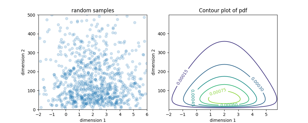
Sample the distribution and plot the pdf of the distribution.

In a similar manner to univariate distributions, samples can be drawn from an JointIndependent distribution using its rvs method.

data = dist.rvs(nsamples=1000)
fig, ax = plt.subplots(ncols=2, figsize=(10, 4))
ax[0].scatter(data[:, 0], data[:, 1], alpha=0.2)
ax[0].set_xlabel('dimension 1')
ax[0].set_ylabel('dimension 2')
ax[0].set_title('random samples')
ax[0].set_ylim([0, 500])
ax[0].set_xlim([-2, 6])

x = np.arange(-2.0, 6.0, 0.2)
y = np.arange(0.01, 500, 1)
X, Y = np.meshgrid(x, y)
Z = dist.pdf(x=np.concatenate([X.reshape((-1, 1)), Y.reshape((-1, 1))], axis=1))
CS = ax[1].contour(X, Y, Z.reshape(X.shape))
ax[1].clabel(CS, inline=1, fontsize=10)
ax[1].set_xlabel('dimension 1')
ax[1].set_ylabel('dimension 2')
ax[1].set_title('Contour plot of pdf')
ax[0].set_ylim([0, 500])
ax[0].set_xlim([-2, 6])
plt.show()

Print the moments of the distribution

Providing a single or multiple consecutive initials of the following four distributions moments ‘m’: mean, ‘v’: variance, ‘s’: skewness, ‘k’: kurtosis allows the user to obtains the respective moments from all underlying univariate distributions. In the following examples providing the string ‘mv’ to the moments function, returns the respective means and variances.

print(dist.moments())
print(dist.moments(moments2return='mv'))

(array([  2.        , 244.69193226]), array([4.0000000e+00, 1.0288065e+05]), array([0.        , 6.18487714]), array([  0.        , 110.93639218]))
(array([  2.        , 244.69193226]), array([4.0000000e+00, 1.0288065e+05]))

Modify the parameters of the distribution.

Use the update_parameters method.

print(dist)
print()
print('Parameters of the marginals:')
print([m.parameters for m in marginals])
print('Parameters of the joint:')
print(dist.get_parameters())
print()
print('Update the location parameter of the second marginal and scale parameter of first marginal...')
dist.update_parameters(loc_1=1., scale_0=3., )
print('Parameters of the marginals:')
print([m.parameters for m in marginals])
print('Parameters of the joint:')
print(dist.get_parameters())

<UQpy.distributions.collection.JointIndependent.JointIndependent object at 0x74d188e8ee20>

Parameters of the marginals:
[{'loc': 2.0, 'scale': 2.0}, {'s': 1.0, 'loc': 0.0, 'scale': 148.4131591025766}]
Parameters of the joint:
{'loc_0': 2.0, 'scale_0': 2.0, 's_1': 1.0, 'loc_1': 0.0, 'scale_1': 148.4131591025766}

Update the location parameter of the second marginal and scale parameter of first marginal...
Parameters of the marginals:
[{'loc': 2.0, 'scale': 3.0}, {'s': 1.0, 'loc': 1.0, 'scale': 148.4131591025766}]
Parameters of the joint:
{'loc_0': 2.0, 'scale_0': 3.0, 's_1': 1.0, 'loc_1': 1.0, 'scale_1': 148.4131591025766}