Morris Screening
Consider a model of the sort \(Y=h(X)\), \(Y\) is assumed to be scalar, \(X=[X_{1}, ..., X_{d}]\).
For each input \(X_{k}\), the elementary effect is computed as:
where \(\Delta\) is chosen so that \(X_{k}+\Delta\) is still in the allowable domain for every dimension \(k\).
The key idea of the original Morris method is to initiate trajectories from various “nominal” points X randomly selected over the grid and then gradually advancing one \(\Delta\) at a time between each model evaluation (one at a time OAT design), along a different dimension of the parameter space selected randomly. For \(r\) trajectories (usually set \(r\) between 5 and 50), the number of simulations required is \(r (d+1)\).
Sensitivity indices are computed as:
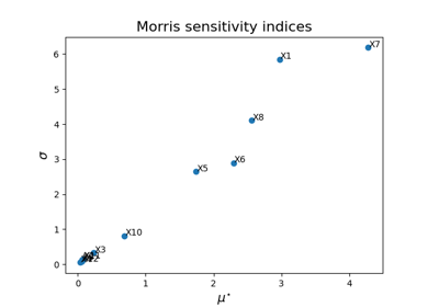
It allows differentiation between three groups of inputs: - Parameters with non-influential effects, i.e., the parameters that have relatively small values of both \(\mu_{k}^{\star}\) and \(\sigma_{k}\). - Parameters with linear and/or additive effects, i.e., the parameters that have a relatively large value of \(\mu_{k}^{\star}\) and relatively small value of \(\sigma_{k}\) (the magnitude of the effect \(\mu_{k}^{\star}\) is consistently large, regardless of the other parameter values, i.e., no interaction). - Parameters with nonlinear and/or interaction effects, i.e., the parameters that have a relatively small value of \(\mu_{k}^{\star}\) and a relatively large value of \(\sigma_{k}\) (large value of \(\sigma_{k}\) indicates that the effect can be large or small depending on the other values of parameters at which the model is evaluated, ndicates potential interaction between parameters).

Function with nonlinearities / parameter dependencies